Exporting to RADMC-3D

New in version 2.6.

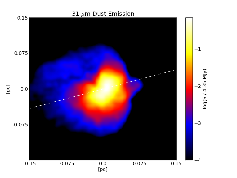
Above: a sample image showing the continuum dust emission image around a massive protostar made using RADMC-3D and plotted with pyplot.

RADMC-3D is a three-dimensional Monte-Carlo radiative transfer code that is capable of handling both line and continuum emission. yt comes equipped with a RadMC3DWriter class that exports AMR data to a format that RADMC-3D can read. Currently, only the ASCII-style data format is supported. In principle, this allows one to use RADMC-3D to make synthetic observations from any simulation data format that yt recognizes.

Continuum Emission

To compute thermal emission intensities, RADMC-3D needs several inputs files that describe the spatial distribution of the dust and photon sources. To create these files, first import the RADMC-3D exporter, which is not loaded into your environment by default:

import yt
import numpy as np
from yt.extensions.astro_analysis.radmc3d_export.api import RadMC3DWriter, RadMC3DSource

Next, load up a dataset and instantiate the RadMC3DWriter. For this example, we’ll use the “StarParticle” dataset, available here.

ds = yt.load("StarParticles/plrd01000/")
writer = RadMC3DWriter(ds)

The first data file to create is the “amr_grid.inp” file, which describes the structure of the AMR index. To create this file, simply call:

writer.write_amr_grid()

Next, we must give RADMC-3D information about the dust density. To do this, we define a field that calculates the dust density in each cell. We assume a constant dust-to-gas mass ratio of 0.01:

dust_to_gas = 0.01


def _DustDensity(field, data):
    return dust_to_gas * data["density"]


ds.add_field(("gas", "dust_density"), function=_DustDensity, units="g/cm**3")

We save this information into a file called “dust_density.inp”.

writer.write_dust_file(("gas", "dust_density"), "dust_density.inp")

Finally, we must give RADMC-3D information about any stellar sources that are present. To do this, we have provided the RadMC3DSource class. For this example, we place a single source with temperature 5780 K at the center of the domain:

radius_cm = 6.96e10
mass_g = 1.989e33
position_cm = [0.0, 0.0, 0.0]
temperature_K = 5780.0
star = RadMC3DSource(radius_cm, mass_g, position_cm, temperature_K)

sources_list = [star]
wavelengths_micron = np.logspace(-1.0, 4.0, 1000)

writer.write_source_files(sources_list, wavelengths_micron)

The last line creates the files “stars.inp” and “wavelength_micron.inp”, which describe the locations and spectra of the stellar sources as well as the wavelengths RADMC-3D will use in it’s calculations.

If everything goes correctly, after executing the above code, you should have the files “amr_grid.inp”, “dust_density.inp”, “stars.inp”, and “wavelength_micron.inp” sitting in your working directory. RADMC-3D needs a few more configuration files to compute the thermal dust emission. In particular, you need an opacity file, like the “dustkappa_silicate.inp” file included in RADMC-3D, a main “radmc3d.inp” file that sets some runtime parameters, and a “dustopac.inp” that describes the assumed composition of the dust. yt cannot make these files for you; in the example that follows, we used a “radmc3d.inp” file that looked like:

nphot = 1000000
nphot_scat = 1000000

which basically tells RADMC-3D to use 1,000,000 photon packets instead of the default 100,000. The “dustopac.inp” file looked like:

2
1
-----------------------------
1
0
silicate
-----------------------------

To get RADMC-3D to compute the dust temperature, run the command:

./radmc3D mctherm

in the directory that contains your “amr_grid.inp”, “dust_density.inp”, “stars.inp”, “wavelength_micron.inp”, “radmc3d.inp”, “dustkappa_silicate.inp”, and “dustopac.inp” files. If everything goes correctly, you should get a “dust_temperature.dat” file in your working directory. Once that file is generated, you can use RADMC-3D to generate SEDs, images, and so forth. For example, to create an image at 31 microns, do the command:

./radmc3d image lambda 31 sizeau 30000 npix 800

which should create a file called “image.out”. You can view this image using pyplot or whatever other plotting package you want. To facilitate this, we provide helper functions that parse the image.out file, returning a header dictionary with some useful metadata and an np.array containing the image values. To plot this image in pyplot, you could do something like:

import matplotlib.pyplot as plt
import numpy as np
from yt.extensions.astro_analysis.radmc3d_export.api import read_radmc3d_image

header, image = read_radmc3d_image("image.out")

Nx = header["Nx"]
Ny = header["Ny"]

x_hi = 0.5 * header["pixel_size_cm_x"] * Nx
x_lo = -x_hi
y_hi = 0.5 * header["pixel_size_cm_y"] * Ny
y_lo = -y_hi

X = np.linspace(x_lo, x_hi, Nx)
Y = np.linspace(y_lo, y_hi, Ny)

plt.pcolormesh(X, Y, np.log10(image), cmap="hot")
cbar = plt.colorbar()
plt.axis((x_lo, x_hi, y_lo, y_hi))
ax = plt.gca()
ax.set_xlabel(r"$x$ (cm)")
ax.set_ylabel(r"$y$ (cm)")
cbar.set_label(r"Log Intensity (erg cm$^{-2}$ s$^{-1}$ Hz$^{-1}$ ster$^{-1}$)")
plt.savefig("dust_continuum.png")

The resulting image should look like:

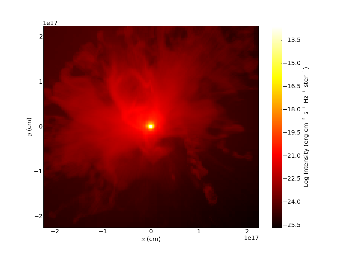
This barely scratches the surface of what you can do with RADMC-3D. Our goal here is just to describe how to use yt to export the data it knows about (densities, stellar sources, etc.) into a format that RADMC-3D can recognize.

Line Emission

The file format required for line emission is slightly different. The following script will generate two files, one called “numderdens_co.inp”, which contains the number density of CO molecules for every cell in the index, and another called “gas-velocity.inp”, which is useful if you want to include doppler broadening.

import yt
from yt.extensions.astro_analysis.radmc3d_export.api import RadMC3DWriter

x_co = 1.0e-4
mu_h = yt.YTQuantity(2.34e-24, "g")


def _NumberDensityCO(field, data):
    return (x_co / mu_h) * data["density"]


yt.add_field(("gas", "number_density_CO"), function=_NumberDensityCO, units="cm**-3")

ds = yt.load("IsolatedGalaxy/galaxy0030/galaxy0030")
writer = RadMC3DWriter(ds)

writer.write_amr_grid()
writer.write_line_file(("gas", "number_density_CO"), "numberdens_co.inp")
velocity_fields = ["velocity_x", "velocity_y", "velocity_z"]
writer.write_line_file(velocity_fields, "gas_velocity.inp")